Quantum Computing I: A Universal Quantum Computer

References

• "Quantum Computation and Quantum Information" by Nielsen and Chuang. The first two chapters provide a detailed and self-contained introduction and explanation of qubits and quantum gates.
• Lecture notes for the course "Qubits, quantum mechanics, and computers" from Umesh Vazirani at Berkeley.
• Lecture notes from John Preskill at Caltech.
• Lecture notes from Ryan O'Donnell and John Wright at CMU. First and second lectures cover basic quantum mechanics and quantum gates.
• Wikipedia article on qubits.
• Wikipedia article on quantum gates.
• A very rough draft of notes on quantum computing we put together when we were thinking what this course would look like

Minimal Background

States

A quantum state is represented by a vector where each spot in that vector corresponds to a binary number.
The length of the vector is $2^\textrm{number of wires}$

Imagine you have three wires. Then you might have a vector like
$$
\begin{equation}
|\Psi\rangle=\begin{bmatrix}
\sqrt{0.1}, \
\sqrt{0.05}, \
-\sqrt{0.15},\
\sqrt{0.2}, \
0.0, \
-\sqrt{0.25},
\sqrt{0.01},
\sqrt{0.24}
\end{bmatrix}
\end{equation}
$$

You could also represent this as
$$ |\Psi\rangle =\sqrt{0.1} |000\rangle + \sqrt{0.05}|001\rangle + -\sqrt{0.15}|010\rangle + \sqrt{0.2}|011\rangle +-\sqrt{0.25}|101\rangle + ...$$

Notice that $|\Psi\rangle ( |\Psi\rangle)^{T*}$ have to add up to 1.
We could also write this as $\langle \Psi | \Psi \rangle$

This tell us that the three wires are in a superposition such that

• the three wires have a $\sqrt{0.1}$ amount of being all zero (i.e. 000).
• the three wires have a $\sqrt{0.15}$ amount of having the middle wire be 1 and the outer wires be 0 (i.e. 010)
• etc.

A quantum gate changes the state of the quantum system. While we might write a quantum gate on one wire, it's sneakily actually a gate on all three wires; it just does nothing on the wires that we don't write it on (the gate is applying the identity operator). The application of a quantum gate multiplies the quantum state by a matrix (padded by the relevant identities).

We can think of a single quantum gate either in the context of its matrix or its application to a qubit:

Hadamard
\[ H=\frac{1}{\sqrt{2}}\left[ \begin{bmatrix} 1 & 1 \\ 1 & -1 \end{bmatrix} \right] \]

$$
\begin{equation}
|0\rangle \rightarrow \frac{1}{\sqrt{2}}(|0\rangle + |1\rangle) \\
|1\rangle \rightarrow \frac{1}{\sqrt{2}}(|0\rangle - |1\rangle)
\end{equation}
$$

Phase($\theta$)
\[ H=\left[ \begin{bmatrix} 1 & 0 \\ 0 & e^{i\theta} \end{bmatrix} \right] \]

$$
\begin{equation}
|0\rangle \rightarrow |0\rangle \\
|1\rangle \rightarrow e^{i\theta}|1\rangle
\end{equation}
$$

CNOT
\[ H=\left[ \begin{bmatrix} 1 & 0 & 0 & 0 \\ 0 & 1 & 0 & 0 \\ 0 & 0 & 0 & 1\\ 0 & 0 & 1 & 0\\ \end{bmatrix} \right] \]
$$
\begin{equation}
|00\rangle \rightarrow |00\rangle \\
|01\rangle \rightarrow |01\rangle \\
|10\rangle \rightarrow |11\rangle \\
|11\rangle \rightarrow |10\rangle\\
\end{equation}
$$

Simulator Ia

In this section, you will build a simulator which takes a description of a quantum circuit and then gives an output. The description of your quantum circuit will have a number of gates (H, CNOT, P) and possibly a measurement at the end.

Input $\xrightarrow{Quantum Circuit}$ Quantum State $\xrightarrow{Measurement}$ Probabilistic Binary Output
$|000\rangle$ $\xrightarrow{Quantum Circuit}$ $ \sqrt{0.2} |000 \rangle + \sqrt{0.3} |101\rangle + \sqrt{0.5}|111\rangle$ $\xrightarrow{Measurement}$ $|101\rangle$

Input: By default the input of your quantum computing simulator will be $|00..00\rangle$. Later on you will add a feature that lets you input another state (this will be useful for debugging).
(Q: What is the vector for the state $|000\rangle$?)

Description: Here is an example of a description of your quantum circuit.

1
2
3
4
5
6
7
8

3
H 1
H 2
P 2 0.3
CNOT 2 1
H 1
H 2
CNOT 2 0

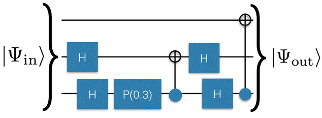
This block says that you have a circuit with 3 wires (the first line) with a Hadamard gate on wire 1 and 2, a phase gate with angle $\theta=0.3$ radians, a CNOT gate between wires 2 and 1, then another two Hadamards and another CNOT. The fact that the CNOT says “2 0” means that the 2 is the control wire. Graphically it would look like this:

This particular circuit should output
$$(0.977668244563+0.147760103331j)|000 \rangle + (0.0223317554372-0.147760103331j)|101 \rangle$$

(Work this out by hand and convince yourself of that.)

If instead our description had a measurement at the end like

1
2
3
4
5
6
7
8
9

3
H 1
H 2
P 2 0.3
CNOT 2 1
H 1
H 2
CNOT 2 0
MEASURE

then the output is probabilistic. $97.76\%$ of the time it will output the state "$|000\rangle$" and $2.23\%$ of the time it will output the state $|101\rangle$.

Although your quantum computing simulator will be able to run without MEASURE at the end, in the real world quantum computers always have a measurement at the end.

• A general circuit can be represented by a unitary matrix $U_\textrm{circuit}.$ From a description of the circuit, build this matrix. Then:
  • Generate the vector for the input $|\Psi_\textrm{in}\rangle = |00..0\rangle$ (n zeros). This is a quantum state and quantum states are represented in your program by a $2^n$ size vector where $n$ is the number of wires.
  • Multiply the vector $|\Psi_\textrm{in}\rangle$ by $U_\textrm{circuit}$. This gives you the output quantum state $|\Psi_\textrm{out}\rangle$
  • Measure the final quantum state $|\Psi_\textrm{out}\rangle.$ This is done by returning the binary number $\langle ij..k |$ with probability $|\langle ij..k |\Psi_\textrm{out}\rangle|^2$. (Figure out what this means in terms of your vector)

There is a convention about whether wire "0" affects the most significant bit or the least significant bit. You should use the convention that it affects the most significant bit!

Constructing the unitary matrix for the quantum circuit.

To make matrix representations of $n$-wire circuits, you first need to understand how to make matrix representations of the circuit components which act on 1 or 2 wires.

Let’s start by thinking about the Hadamard gate. I want to accomplish this:

The input state is $\sqrt{0.3}|0\rangle + \sqrt{0.7}|1\rangle$. First, figure out how to represent this state as a vector. Then figure out what the output vector should be after its application.

As a next step, figure out how to build the unitary matrix for this quantum circuit:

Notice that this is the same input state (do you understand why?), though now it is represented by a $2^3$ size vector. (What is the $2^3$ size vector for this state?). The unitary matrix representing this quantum circuit is $2^3 \times 2^3$ even though the Hadamard gate applies only to the first wire. A trick for constructing the larger representation is to build the matrix $I \otimes H \otimes I$, where $H$ is the matrix for the Hadamard gate, $I$ is an identity matrix, and $\otimes$ denotes a tensor product. Write code that constructs the matrix representing a Hadamard applied to wire $i$ in a $k$-wire circuit (in this case $k=3$). Working in python, you might define a function that looks something like this

1
2
3
4
5
6

    def HadamardArray(i, k):
      # this should apply Hadamard to wire i out of k wires
      size=...
      myMatrix=numpy.zeros((size,size))
      #do stuff
     return myMatrix

Python hint: a @ b multiplies two matrices (or numpy arrays)

Repeat this exercise for the phase gate (note, to construct the array your function will need the phase angle as an argument). Begin by figuring out the correct matrix for the phase gate on one wire.

I found it useful to build a function tensorMe(listOfMatrices) which takes a list of matrices and generates their tensor product.

The CNOT gate: The next step in building our simulator is to construct matrix representations for gates that act on multiple wires. The controlled-not gate, CNOT, is non-trivial because it is applied to two wires at once.

We have told you what the right matrix to use for a right-side up CNOT. Figure out the right matrix to multiply your state for an upside-down CNOT on the left of the gate $|\Psi_\textrm{left}\rangle$ by to get the state on the right of the gate $|\Psi_\textrm{right}\rangle$.

Now, let’s figure out how to do it when the CNOT gate is in the middle of four wires, like below.

Remember, you are going to use identities to tensor against this. You will want to write a function like

1
2
3
4

    def CNOTArray(controlWire,otherWire,totalWires):
      myMatrix=numpy.zeros((size,size))
      #do stuff
     return myMatrix

Test your function after you’ve written it. You can make some input state and verify that it produces the correct output state, like below.

1
2

    myInputState = ... #some state of 4 wires
    myOutputState = CNOTArray(3,2,4)* myInputState

Make sure to check your results by hand.

A challenge: We’ve figured out how to construct CNOT gates that apply to neighboring wires. But what happens if the controlled bit is further away from the controlling bit (say between wires 1 and 3), like such:

Can you figure out how to write the matrix for this gate? This is much harder then the other things you’ve done. If you can get it to work, that’s great. If not, don’t worry about it. We’ll see in a couple minutes how to do it.

Putting the gates together: You’ve figured out how to make matrix representations for various gates. Now suppose we want to compose multiple gates into a more complete circuit. For example, suppose you have the following input

1
2
3
4

    3
    H 1
    CNOT 1 2 
    P 0 0.45

It consists of three gates applied sequentially. You know how to build the matrix for each of these individual gates (in the dotted boxes).

Let’s now proceed with building the unitary matrix which represents this circuit. Be careful about the order in which you apply your matrices; remember that the input travels from left to right.

At this point, you (personally) should be able to take a circuit description and produce the unitary circuit which represents it. The next step is to configure your program to read the input from a file and build the matrix automatically. Parsing input is a bit annoying, so we’re happy to give you this piece. Go ahead and use the following if you want.

1
2
3
4
5
6
7

    def ReadInput(fileName):
        myInput_lines=open(fileName).readlines()
        myInput=[]
        numberOfWires=int(myInput_lines[0])
        for line in myInput_lines[1:]:
            myInput.append(line.split())
        return (numberOfWires,myInput)

Then you can read the gate by doing

1
2
3
4

    myInput=ReadInput("myGateDescription")
    firstGate=myInput[0][0]
    secondGate=myInput[1][0]
    firstWire=myInput[0][1]

At this point you should be able to take a circuit description (without measurement) and print out the quantum state of the system at the end. You should be using your pretty print functions to print this out in a nice way using Dirac notation.

Measuring

Your next step should be to get measurement working. When you measure at the end your code should output binary number $|i\rangle$ with probability $|\langle i | \Psi_\textrm{out}\rangle|^2$. Modify your simulator so that it can correctly produce the result with measurement.

Input

By default we will assume that the input to your quantum circuit is the state $|00..0\rangle$. Often (especially for testing purposes) you'll want to be able to put in another input though. To do this, we will use a line like

INITSTATE FILE myInputState

where myInputState will be a file with $2^n$ complex numbers in it like such:

0.0 -0.0
0.0 -0.0
0.0 -0.0
0.0 -0.7071
0.0 -0.0
0.0 -0.0
0.7071 0.0
0.0 -0.0

for the state $\frac{1}{\sqrt{2}} \left( -i |3\rangle + |6 \rangle\right)$

Also, you should be able to read inputs like

INITSTATE BASIS |001>

Congrats! At this point you should have a basic working simulator.

Grading

Hopefully at this point you've tested your simulator and are convinced that it works. To grade your simulator, we will run it on a number of inputs below. You should paste your results to these outputs into your document. One of our inputs has a MEASURE at the end. For this input you should produce a graph which is a histogram of output versus counts. Tests: rand.circuit measure.circuit input.circuit myInputState

Computational Complexity

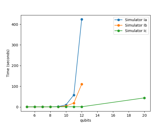
One of the reoccuring themes in this course will be using efficient algorithms. Let's think about the efficiency of our simulation. There are two things we might consider: the time complexity and the space complexity. Let $g$ be the number of gates and $2^w=N$ be the size of the Hilbert space. You needed to make $g$ matrices with $N^2$ numbers in them. Therefore, the amount of space that you took up was something like $gN^2$ (depending on how you implemented things it might even be just $O(N^2)$ RAM). In terms of your complexity, you needed to multiply a bunch of $N \times N $ matrices. Each such multiplication takes $O(N^3)$ work. So you needed to do something like $gN^3$ work.

Simulator Ib

Note: You are going to improve your algorithm here. Don't erase your old version because although it is slower it gives you more information that you will sometimes find useful.

Let's go ahead and make some minor changes that will improve the efficiency of the algorithm.

We can significantly decrease the amount of work if we build the matrix for the first circuit element and then multiply by the current state to produce the output state. Then you can build the matrix for the next gate and multiply it against the current state. Go ahead and do this. Now, applying each gate involves a matrix-vector multiplication. That takes $O(N^2)$ time each for a total time of $O(gN^2)$. You stil need $O(N^2)$ RAM.

	Grading
	Do the same tests as above on your faster simulator and paste them into your document.

Simulator Ic

Once you have this implemented, let's make another improvement. Currently, you are building big matrices for each gate. Q: How many non-zero elements does your matrix actually have? What you will find is that it should only have $O(N)$ non-zeros. This suggests that we should store the matrices in a sparse way. Build up your matrix, then using sparse matrices. You might want to use scipy.sparse.kron for doing this. Allow the vector to be dense but do the matrix-vector product using sparse matrices. The total RAM you are using is now $O(N)$. Also, each matrix-vector multiplication, only involves $O(N)$ work. This is much better.

You want to make everything sparse and keep it sparse. The trick is to use scipy.sparse to keep everything in csr format.
I used commands like (not in this order)

scipy.sparse.csr_matrix(scipy.sparse.identity(1,dtype='complex'))
myState.tocsr()
scipy.sparse.kron(myMatrix,matrix,format='csr')
scipy.sparse.csr_matrix([[1,0],[0,numpy.exp(1.j*theta)]])

Using a @ b keeps everything sparse in python.

Grading

Do the same tests as above to verify your simulator works. You should measure the time that both simulators takes as a function of number of qubits. Generate random circuits of a fixed length with more and more qubits and see how long things take by running time python mySimulator.py myInput. Make a plot of the result like below and add it to your document. Do the same thing with the RAM (use top or activity monitor to view the ram usage. You just need to get an approximation)