Part I: Simulating an Ising Model

In this page, you will write Monte Carlo code to sample configurations from the Ising model with the correct probability.

Minimal background

The Ising model

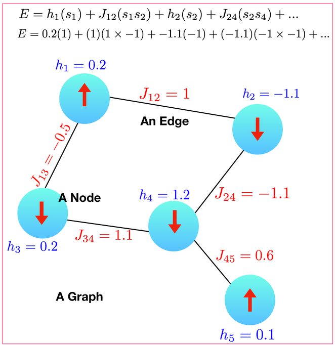
The Ising model is one of the drosophila of physics. At first look, it's a simple model of crystalline materials which attributes magnetism to the orientation of magnetic moments on a lattice, summarized by the Hamiltonian or energy

$$
E = - \sum_{i,j} J_{ij} s_i s_j + \sum_i h_i s_i.
$$

The variables $s_i$ express the possible orientations for each moment, while the entries $J_{ij}$ of the (symmetric) interaction matrix characterize the interaction energy of moments $i$ and $j$. The value $h_i$ specifies a magnetic field on each site $i$.

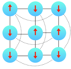
Ising's original formulation (often referred to as the Ising model) considers moments with two orientations, $s_{i} = \pm 1$, which only interact with their nearest neighbors, $J_{ij} = J \delta_{j,i+1}$ with $J$ constant and $h_i=0$. Below we will call this the two-dimensional Ising model.

A configuration of an Ising model is a specification of every moment's orientation — an assignment of values to the $s_i$ variable for all moments in the system. For our purposes, configurations are 'snapshots' of the system which our simulator will hold in memory, like a vector containing $\pm 1$ in its $i$th entry to specify whether moment $i$ points up or down.

Statistical Mechanics

There are a couple facts we need to know about statistical mechanics.

(1) We can specify configurations of our system $c.$ In the case of an Ising model, the configuration is the orientation of each spin.

(2) Each configuration $c$ has an energy $E(c)$. We've already seen this for the Ising model.

(3) For classical systems in contact with an energy reservoir of temperature $T$, the probability $P$ of finding the system in configuration $c$ is
$$P(c) = \frac{e^{-\beta E(c)}}{\sum_c e^{-\beta E(c)}}$$
where $E(c)$ is the configuration's energy and $\beta \equiv 1/(kT)$ with $k$ Boltzmann's constant and $T$ is the temperature. We will work in units where $k=1.$

Markov Chains

We have just learned that statistical mechanics tells us that if we look at the system, each configuration $c$ appears with probability $P(c)\sim \exp(-\beta E(c))$. Our first goal is to implement an algorithm which gives us configurations $c$ with probability $P(c)$.

One such algorithm is markov chain Monte Carlo.

A Markov chain is a process where you are at some state $c$ (i.e. a configuration) and then you choose another state $c'$ with a probability that only depends on $c$. In other words, you can't use the fact that previously you were at configuration $b$ to decide the probability $P(c \rightarrow c')$ you're going to go from $c$ to $c'$. This process is called a memoryless process.

As long as you do a (non-pathalogical) random walk in a memoryless way, you're guaranteed that, after walking around enough, that the probability you are in configuration $c$ is some $\pi(c)$. $\pi$ is called the stationary distribution. Different markov chains will have different stationary distributions. A Markov chain is non-pathological if:

• It is aperiodic; it doesn't cycle between configurations in a subset of the system's full configuration space.
• It is connected; given two configurations, there is a path with non-zero probability that the chain could (but not necessarily will) follow to get from one to the other.

To simulate the Ising model, we wish to build a markov chain which has the stationary distribution $\pi(c) \sim \exp(-\beta E_c)$. We will do so with a very famous algorithm which lets us build a Markov chain for any $\pi(c)$ we want.

The Metropolis-Hastings algorithm

If you know your desired stationary distribution, the Metropolis-Hastings algorithm provides a canonical way to generate a Markov chain that produces it. The fact that you can do this is amazing! The steps of the algorithm are:

• Start with some configuration $c$
• Propose a move to a new trial configuration $c'$ with a transition probability $T(c\rightarrow c')$
• Accept the move to $c'$ with probability $\min \left(1, \frac{\pi(c')}{\pi(c)}\frac{T(c'\rightarrow c)}{T(c \rightarrow c')} \right)$

The first step is straightforward, but the latter two deserve some explanation.

How $T(c\rightarrow c')$ is picked: Choosing a procedure for movement between configurations is the art of MCMC, as there are many options with different strengths and weaknesses. In the simplest implementations of the Metropolis algorithm we choose a movement procedure where forward and reverse moves are equiprobable, $T(c \rightarrow c') = T(c' \rightarrow c)$.

Question to think about: How do equiprobable forward and reverse moves simplify the Metropolis algorithm?

Acceptance condition: To construct a Markov chain which asymptotes to the desired distribution $\pi$, the algorithm must somehow incorporate $\pi$ in its walk through configuration space. Metropolis does this through the acceptance ratio

$$
\alpha \equiv \frac{\pi(c')}{\pi(c)}\frac{T(c'\rightarrow c)}{T(c \rightarrow c')}.
$$

Notice how the first factor in $\alpha$ is the relative probability of the configurations $c'$ and $c$. Assuming that $T(c \rightarrow c')=T(c' \rightarrow c)$, we have that $\alpha > 1$ indicates that $c'$ is more likely than $c$, and the proposed move is automatically accepted. When $\alpha < 1$, $c'$ is less probable than $c$, and the proposed move is accepted with probability $\alpha$.

Question to think about: Why are moves with $\alpha < 1$ accepted with probability $\alpha$, rather than outright rejected?

Writing your simulation

State and Parameters

The first thing to do is to figure out how to store the configuration $c$ as well as the coupling constants $J_{ij}$ and $h_i.$ There are two options to go about this. Option 1 is much simpler and all you will need for this assignment! Only do option 2 if you want a more general code and feel like you know what you're doing.

Option 1: Suppose we are only interested in running the two-dimensional Ising model on a square grid (which will be our primary concern). Then the simplest thing might be to put the state of the spins in a two dimensional array and store a single value of $J$. There are two approaches to storing the two dimensional array. One approach is to use the STL: vector<vector<int> > spins. Another option is to use Eigen (see here) where you will use MatrixXi. The advantage of option 1 is it is easy to think about. There are two down-sides though. First, you have to do some gymnastics to worry about the periodic boundary conditions (i.e. the node to your left is something like (i+spins.size()+1) % spins.size(), etc). Secondly, you don't have a lot of flexibility. Suppose you want to be on a triangular lattice instead of a square; have a different $J$ for every bond; or change the boundary conditions. You'd end up having to write a bunch of different code to represent your spins.

Option 2:

A more general way to store your configuration is to put your spins (and magnetic field) on nodes of a graph and the coupling constants $J_{ij}$ as edges.

A graph has a bunch of nodes (each node $i$ has a state $s_i$ which is either spin-up or spin-down and has a magnetic field $h_i$) and a bunch of edges (each edge has a $J_{ij}$ on it). Then, if you want a grid you can just choose a graph that is grid-like.

Now there are two questions: how do you represent this inside your code and how do you get the code to know about the graph that you want.

Representing your spins: Here is what I did in my code. I wrote an Ising class which has two vectors which represent the state of the nodes and their magnetic fields (i.e. vector<int> spins and vector<double> h). Then, I stored a neighbor vector. The i'th element in the neighbor vector stores a list (or vector) of neighbors with their respective coupling constants.
In other words, for the graph above, you want to be storing the following inside your computer:

Node: (neighbor, J)  (neighbor, J) (neighbor, J) ...
1: (2, 1)  (3,-0.5)
2: (1,1)  (4,-1.1)
3: (1,-0.5) (4,1.1)
4: (2,-1.1) (3,1.1) (5,0.6)
5: (4,0.6)

I stored this as vector<vector<pair<int, double> > > neighbors where the pair<int,double> stores the node you are a neighbor to and the weight.

Setting up your graph: Setting up your Ising model this way gives you a lot of flexibility. But now you need some way to tell your code what particular graph you want (maybe the one above or a grid, etc).

I recommend doing this by reading two files. A "spins.txt" which tells you the value of $h_i$ for spin $i$ and a "bonds.txt" which tells you which spins are connected and what their coupling constants are.

For the first graph above:
bonds.txt

1 2 1.0
1 3 -0.5
3 4 1.1
2 4 -1.1
4 5 0.6

spin.txt

1 0.2
2 -1.1
3 0.2
4 1.2
5 0.1

Then just write some sort of Init() function for your Ising model to read in the graph. Also, go ahead and write yourself a python code that generates the relevant graph for a two-dimensional Ising model on a square grid. Now, any time you want to run a different Ising model, you just have to change these files.

Computing the Energy

No matter which option you chose, the next step in putting together your Ising model is learning how to compute the energy $E(c)$ of a configuration. Write some code (i.e double Energy()) which allows you to do this.

For debugging and analysis purposes, it's going to be helpful to get your code to read and write spin configurations. You should add a 'string toString()' which returns a string representing the configuration of your Ising model and void fromString(string &myString) which eats a string and sets up your Ising model with that string.

In addition to computing the energy for a single configuration, it's going to be useful to be able to compute the energy difference between two configurations that differ by a single spin flip (i.e. double deltaE(int spin_to_flip)) Why is this? Because the acceptance criterion we are going to use is the ratio of $\exp[-\beta E_\textrm{new}]/\exp[-\beta E_\textrm{old}]=\exp[-\beta \Delta E]$ Go ahead and make this function.

	Testing
	Set up a $3 \times 3$ grid and compute the energy of some spin configuration both by hand and with your code to make sure it's the same Compute the energy difference of flipping a single spin both by using your Energy() function before and after a spin flip. using your deltaE() function. They should be the same.

Comment about computational complexity: One of the themes of this class is to think about the scaling of your algorithms (like we did thinking about various options for quantum computing). Let's do this for computing an energy difference. One thing you can do is compute the energy, flip the spin, compute the energy, and subtract. How long does this take? It takes $O(N + B)$ time where $N$ is the number of spins and $B$ is the number of bonds. Find a way to do it with a time that is proportional to $O(1)$ when you have a grid.

At this point you should be able to store a configuration of spins (with the respective coupling constants) and compute energy and energy differences on them.

Writing MCMC

We now want to put together the Monte Carlo. To go about this, we need to

• Choose a way to go from one configuration to another configuration. The simplest method is to flip a randomly chosen spin. Make sure to compute $T(c\rightarrow c')$ and visa-versa. Let $c'$ be your new configuration (say with the flipped spin) and $c$ be the old configuration.
• If $\frac{T(c' \rightarrow c)}{T(c \rightarrow c')} \frac{\exp[-\beta E(c')]}{\exp[-\beta E(c)]}>\textrm{ran}(0,1)$ then accept the new configuration $c'$. Otherwise leave the old configuration $c$

This needs to happen over and over again. Important point about time-scales: We could just have a loop that picks a spin and flips it over and over and call that a step. In practice, we want to only count things in terms of sweeps: doing $N$ spin-flips. This is because flipping a single spin doesn't change things very much. Therefore, you want:

for (int sweep=0;sweep<10000;sweep++){
    for (int i=0;i<N;i++){
        //Pick a random spin and try to flip it
    }
}

For your $3 \times 3$ grid, run your Monte Carlo and make a histogram of the configurations that you see.

When to take snapshots (or more generally compute observables): The promise of MCMC is that after a "long enough time" $T$, you should get a random sample (we unfortunately don't know $T$ a-priori - it's at least one sweep but could be many sweeps). Roughly you want to measure an observable or add to your histogram every $T$ sweeps.

Q: What happens if you take snapshots too infrequently? You end up just wasting some time. The samples are still independent.

Q: What happens if you take snapshots too frequently? That's a little more subtle. If you take snapshots too soon then you are in trouble. This means that you should wait a fair amount of time before you start measuring snapshots.

If you wait enough time for the first snapshot and then take measurements more frequently then you are still ok. It's just you have to be careful with your errorbars because subsequent snapshots may be correlated.

Later on we will see how to estimate $T$. For this simulation,let's just assume that $T$ is about a sweep. Wait 10 sweeps before you begin measuring snapshots. Then take a snapshot every sweep. Error bars for your histogram: If you have $k$ samples in a bin then your error should be $\sqrt{k}$.

Testing

We need to figure out how to determine if our Monte Carlo is working. To do this, let's figure out the expected histogram you should get. The probability we expect to get is $p(c) = \frac{1}{Z} \exp[-\beta E(c)]$ where $Z = \exp[-\beta E(c)]$. Since we have an energy function we can loop over all the configurations $c$ (hint: loop over binary numbers and convert to configurations), evaluate their energy, compute $p(c)$ and graph it.

	Grading
	Add to your document, a histogram with error bars of the configurations for your $3 \times 3$ two-dimensional grid with the exactly computed curve plotted on top of it. These curves should be the same. If they aren't, then you've done something wrong and need to fix it.

Getting sane input

At this point, you're going to want to start running your Ising model code with a bunch of different input parameters (and write various different output files). To do this, we are going to use input files that looks like this:

beta=0.15
Lx=8
Ly=8
outFile=out_L8_0.15
bondsFile=bonds_8

To read them, use the following header file: input.h. You can read input variables, such as inverse temperature "beta" and the grid size in the x-direction "Lx", using the following code:

1
2
3
4
5
6
7
8
9
10
11
12
13
14
15
16

#include <fstream>
#include "input.h"

using namespace std;

// Read the file called "myInputFile.txt" as an input file stream.
ifstream myFile("myInputFile.txt");

// Using InputClass, read in variables "beta" and "Lx".
InputClass input;
input.Read(myFile);
double beta = input.toDouble(input.GetVariable("beta"));
int Lx      = input.toInteger(input.GetVariable("Lx"));

// Close the file stream when done reading input.
myFile.close();

You will need this to work in order to do the number of runs you need to do in the next pages.