
In this section, we will build a feedforward neural network and use it to study phase transitions in the Ising model.
A feedforward neural network is an artificial neural network that has been used extensively to accomplish a wide variety of machine learning tasks. Due to the success of these networks, and their generalizations such as convolutional neural networks, in engineering problems such as image recognition, scientists have begun looking at these networks as potential new tools to study physical phenomenon. In particular, the authors of this paper proposed to use feedforward neural networks to study classical phase transitions. They trained neural nets to identify the magnetic phase transition in the Ising model that we studied in the earlier unit. Our goal is to roughly reproduce the results of this paper and see how neural networks can help us study physics.
Unlike Hopfield networks and restricted Boltzmann Machines, feedforward neural networks are not Ising models. Nonetheless, they still have neurons, weights, and biases.
There are a number of differences, though:
Comment on implementation: When writing up your neural network, it is possible to perform all of the calculations using for loops. However, if you are willing, it is worth trying to perform the calculations with matrix-vector multiplications. This can greatly simplify your code, since nested for loops can be replaced with a few lines of matrix-vector manipulations, and can speed up your code significantly, since matrix-vector libraries are highly optimized. While the C++ standard library does not include matrix-vector functionality, there is a (relatively) easy-to-use library called Eigen that allows you to work with matrices in C++. A handy reference for Eigen commands, and their equivalent commands in Matlab, is available here.
To illustrate how a feedforward neural network produces output from input and introduce the notation, we will first describe a single layer network.
In the above diagram, the graph represent the calculations performed in one layer of the neural network. The nodes in the bottom layer of the graph are input neurons $x_j$ and the nodes at the top are output neurons $z_k$. The neuron variables are evaluated in the order $x_j \longrightarrow y_k \longrightarrow z_k$. There are $m$ input variables $x_j$, $n$ intermediate variables $y_k$, and $n$ output variables $z_k$. The input neurons are connected to the output neurons by the $m \times n$ weight matrix $W_{jk}$ and each output neuron has a bias term $b_k$. The function $f(y)$, called the activation function, adds non-linearity to the model, making it "more expressive" and hopefully able to model non-linear relationships in real data. A commonly used activation function is the sigmoid (or logistic) function $f(y)=1/(1+e^{-y})$.
In summary, the layer takes inputs ${x_j}$ and outputs
$$z_k = f\left(\sum_{j} W_{jk} x_j + b_k \right)$$
Notice, also there are a number of derivatives that you might take of a layers output with respect to
Now, let's write some code that correctly deals with layers. I recommend having a class LayerClass { }; which stores
MatrixXd Weights; ,VectorXd bias,int layer; (i.e am I layer 0 or 1 or 2 or ...)nm.Then we need to include in our class a way to take an input and give the output of the layer (i.e. void evaluate(VectorXd &input, VectorXd &output) ). Write this function and convince yourself that it works for your one layer.
 |
Grading |
|---|---|
| Come up with a test to show that your one layer evaluates correctly. |
Next, we generalize to $L$ layers and introduce a layer index $l=1,\ldots,L$ to all of our variables.
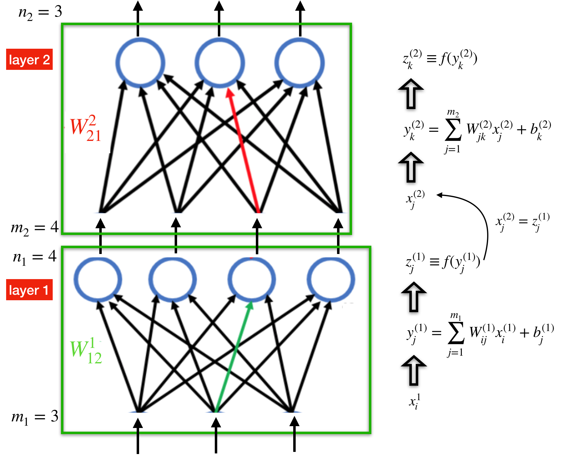
The above diagram shows an $L=2$ layer neural network. The output of layer $l$ is the input to the layer $l+1$ above it, which means that $z^{(l)}=x^{(l+1)}$. Notice that the number of input neurons $m_l$ and the number of output neurons $n_l$ can be different at each layer $l$, but must agree between layers so that $n_l=m_{l+1}$. To compute the output of a many-layer neural network, you just need to follow the arrows up the graph and compute one layer at a time. It is helpful to try to work out a small one- and two-layer neural network out by hand to get a sense of the notation and the calculations involved.
|
Grading |
|---|---|
| Build a neural network which has multiple layers which takes an input and gives out an output. Set up your code so that it can handle arbitary numbers of layers and an arbitrary activation function $f(y)$. Come up with a simple test, for example on a particularly simple or small network, that demonstrates that the output you produce is correct and paste it in your document. |
Feedforward neural networks by themselves are simply highly non-linear functions with many tunable parameters (the weights and biases at each layer). In machine learning contexts, these networks are typically used to perform supervised learning. In supervised learning, the networks are "trained" on labeled data and the network's many parameters are optimized so that the function can accurately predict labels for new data. We will perform this supervised learning on labeled Ising spin configurations.
The task that feedforward neural neural networks are used for is supervised learning. Roughly, the goal of supervised learning is to train a machine to correctly assign labels to unlabeled data. To accomplish this goal, the machine is trained with labeled data, such as images with descriptions of their content. By training on enough high-quality examples, the machine can hopefully learn the underlying structure of the data and then apply its knowledge to data it has not seen before. For a machine learning model to be able to generalize to data it has not seen before, you would expect that the model would need to be "expressive" and have many tunable parameters. Empirically, machine learning researchers have found that neural networks seem to work well on a variety of supervised learning tasks.
Our next goal is to learn how to train our neural network.
In supervised learning, we have a labeled training data set
$$ (x_{s}, \hat{z}_{s}) \quad \textrm{ for } s=1,\ldots,N $$
where $x_s$ is a data point in the data set and $\hat{z}_s$ is its label. In this notation, $x_s$ and $\hat{z}_s$ are vectors.
In the previous section, we learned how to take an input vector $x^{(1)}$ and evaluate an $L$-layer neural network to obtain the output vector $z^{(L)} = z^{(L)}(x^{(1)})$ [This notation is saying that the output at layer $L$ is a function of the input at layer $1$]. After training, we would like our neural network to be able to correctly label the data points in the training data set. What this means is that, for every data point $x_s$, we want our neural network output to match the "true output" as close as possible: $z^{(L)}(x_s) \approx \hat{z}_{s}$.
To quantify this statement, we can compute how different our neural network output is from the true output using a cost function (also called an error function), such as this quadratic function
$$ C(z^{(L)},\hat{z}) = \sum_{k=1}^{n_L}(z_k^{(L)} - \hat{z}_k)^2. $$
There are many possible cost functions that we can use with neural networks. Another one that is often used is the cross-entropy
$$ C(z^{(L)},\hat{z}) = -\sum_{k=1}^{n_L} \hat{z}_k \log z^{(L)}_k - (1-\hat{z}_k) \log(1-z^{(L)}_k) $$
which can be applied when $z^{(L)}_k$ and $\hat{z}_k$ are valid probability distributions, i.e., are normalized to one. In general, which cost function $C$ and activation function $f$ you use in your neural network can significantly affect the efficiency of the network's learning.
The average cost function evaluated on the entire training data set
$$ C = \frac{1}{N} \sum_{s=1}^{N}C(z^{(L)}(x_s), \hat{z}_s) $$
measures how closely our neural network reproduces the labels in the training data. Therefore, our goal in training is to minimize the cost $C$.
To do this, you will also need the derivative of the cost function with respect to the output of your neural network $\partial C/\partial z^L$.
|
Grading |
|---|---|
Write a cost function Cost(VectorXd &z,VectorXd &answer) which takes the output of the neural net and the expected answer as vectors of size $n_L$ and evaluates the cost function. Come up with a way to test this and paste it into your document. Also write a VectorXd& dC_dz(VectorXd &z) which outputs a vector of derivatives where the $k$'th element is $\partial C/\partial z^L_k$. |
Now our goal is to make the average cost function,
$$\langle C \rangle \equiv \sum_{x_0 \in \textrm{inputs } } C(z^L(x_0),A(x_0))$$
smaller (here $A(x_0)$ is the answer we want to get for input $x_0$).
We will do this during training by adjusting the neural network parameters, the weights $W^{(l)}$ and biases $b^{(l)}$ at each layer $l$. How are you going to do this? Well, first we need to notice that, in addition to depending on the input, the neural network's output depends on the network's parameters: $z^{(L)} = z^{(L)}(x^{(1)};W^{(1)},b^{(1)},\ldots, W^{(L)},b^{(L)})$. This means that the average cost function also depends on the network's parameters $C=C(W^{(1)},b^{(1)},\ldots, W^{(L)},b^{(L)})$.
To minimize the cost function in this parameter space, we can use the widely used gradient descent method for minimizing a function. In gradient descent, we iteratively update our parameters by moving them in the direction of the gradient of the objective function we are minimizing. If you imagine the objective function $C$ as a complicated surface with many hills and valleys, then what we do in gradient descent is start at a point on this surface and take steps downhill where the slope is steepest. Of course with this procedure we can get stuck in local minima, but in practice it works well.
In gradient descent, we iteratively update our parameters in the following way:
$$W_{ij}^{(l),new} = W_{ij}^{(l),old} - \eta \frac{\partial C}{\partial W_{ij}^{(l)}} \quad b_{j}^{(l),new} = b_{j}^{(l),old} - \eta \frac{\partial C}{\partial b_{j}^{(l)}}$$
where $\eta$ is a small parameter called the "learning rate" that we are free to choose.
Since we will do this calculation repeatedly, it's important that we be able to compute the gradients ${\partial C}/{\partial W_{ij}^{(l)}}$ and ${\partial C}/{\partial b_{j}^{(l)}}$ efficiently. "Backpropagation" is the name machine learning experts have given to the algorithm for computing the gradients efficiently. While backpropagation has taken on some mystical signficance, in truth it is just a way of taking derivatives smartly by using the chain rule (backpropagation is also a special case of automatic differentiation).
 |
Testing |
|---|---|
| Since backpropagation can be a tricky algorithm to implement correctly, it is important to be able to check that your result is correct. You can do this by implementing another inefficient, but simple, way of computing the gradients ${\partial C}/{\partial W_{ij}^{(l)}}$ and ${\partial C}/{\partial b_{j}^{(l)}}$ called "finite difference", which you can check against backpropagation. In finite difference, you approximate a function's derivative with two closely spaced evaluations of the function: $ \frac{df(x)}{dx} \approx \frac{f(x+\Delta) - f(x)}{\Delta}.$ Applying this to the cost function, you can compute the weight and bias gradients as $ \frac{\partial C}{\partial W_{ij}^{(l)}} \approx \frac{C(W_{ij}^{(l)}+\Delta) - C(W_{ij}^{(l)})}{\Delta} \quad \frac{\partial C}{\partial b_{j}^{(l)}} \approx \frac{C(b_{j}^{(l)}+\Delta) - C(b_{j}^{(l)})}{\Delta}$. Implement the code to do this by finite difference now in preparation for doing backpropagation. |
In this section, we will discuss the backpropagation algorithm for computing the gradients of the cost function. The algorithm consists of two steps, (1) feed forward and (2) backpropagate, which we summarize here.
Feed forward
In this step, you evaluate the neural network from bottom (input) to top (output). The important difference from what you did before is that here you save information as you go up. The information you save will be used in the second step.
Backpropagate
In this step, you evaluate the derivative of the cost function one layer at a time, going from the top to the bottom layer. By using the chain rule, you can use the gradients computed for the upper layers to compute the gradients for the lower layers.
In backpropagation, our goal is to compute the gradients $\partial C/\partial b_j^{(l)}$ and $\partial C/\partial W_{ij}^{(l)}$ for each layer $l=1,\ldots,L$. To understand how to do this, we need to do some algebra. First, let's think about the cost function. For a fixed label $\hat{z}$, our cost function is a sum over the entries of the output vector $z^{(L)}$:
$$ C(z^{(L)}) = \sum_{k=1}^{n_L} c_k(z^{(L)}_k). $$
The first thing that we can do is calculate the gradient of $C$ in the final layer $l=L$. By using the chain rule, we see that the bias gradients in the final layer are:
\[
\begin{aligned}
\frac{\partial C}{\partial b_j^{(L)}} &= \frac{\partial}{\partial b_j^{(L)}} \sum_{j'} c_{j'}(z^{(L)}_{j'}) \newline
&= \sum_{j'} {c'}_{j'}(z^{(L)}_{j'}) \frac{\partial z^{(L)}_{j'}}{\partial b_{j}^{(L)}} \newline
&= \sum_{k'} {c'}_{j'}(z^{(L)}_{j'}) f'(y^{(L)}_{j'}) \frac{\partial y^{(L)}_{j'}}{\partial b_{j}^{(L)}} \newline
&= \sum_{j'} {c'}_{j'}(z^{(L)}_{j'}) f'(y^{(L)}_{j'}) \delta_{jj'} \newline
&= {c'}_{j}(z^{(L)}_{j}) f'(y^{(L)}_{j}) \equiv \delta^{(L)}_j
\end{aligned}
\]
where $c_j'(z) \equiv dc_j(z)/dz$ and $f'(y) \equiv df(y)/dy$ and we introduced a new variable $\delta^{(l)}_j$ to simplify the notation.
Similarly, since $ \partial y^{(L)}_{j'} / \partial W_{ij}^{(L)} = \delta_{jj'} x^{(L)}_i, $ the weight gradients in the final layer are:
\[ \begin{align} \frac{\partial C}{\partial W_{ij}^{(L)}} = {c'}_{j}(z^{(L)}_{j}) f'(y^{(L)}_{j}) x^{(L)}_i = \delta^{(L)}_j x^{(L)}_i \end{align} \]
Next, we will compute the $(L-1)$-th layer gradients. The bias gradients are
\[ \begin{align} \frac{\partial C}{\partial b_j^{(L-1)}} &= \sum_{k'} c'_{k'}(z^{(L)}_{k'}) f'(y_{k'}^{(L-1)}) \frac{\partial y_{k'}^{(L)}}{\partial b_j^{(L-1)}} \newline &= \sum_{k'} \delta^{(L)}_{k'} \frac{\partial}{\partial b_j^{(L-1)}}\left[\sum_{j'}W^{(L)}_{j'k'}x^{(L)}_{j'} + b^{(L)}_{k'} \right] \newline &= \sum_{j'k'} \delta^{(L)}_{k'} W^{(L)}_{j'k'} \frac{\partial x^{(L)}_{j'}}{\partial b_j^{(L-1)}} = \sum_{j'k'} \delta^{(L)}_{k'} \frac{\partial z^{(L-1)}_{j'}}{\partial b_j^{(L-1)}} \newline &= \sum_{j'k'} \delta^{(L)}_{k'} W^{(L)}_{j'k'} f'(y_{j'}^{(L-1)}) \frac{\partial y^{(L-1)}_{j'}}{\partial b_j^{(L-1)}} = \sum_{j'k'} \delta^{(L)}_{k'} W^{(L)}_{j'k'} f'(y_{j'}^{(L-1)}) \delta_{jj'} \newline &= \sum_{k'} \delta^{(L)}_{k'} W^{(L)}_{jk'} f'(y_{j}^{(L-1)}) \equiv \delta^{(L-1)}_j. \end{align} \]
And again, from similar algebra we see that the weight gradients in layer $l=L-1$ are
\begin{align}
\frac{\partial C}{\partial W_{ij}^{(L-1)}} = \delta^{(L-1)}_j x^{(L-1)}_i.
\end{align}
It is very helpful to try to work out some of this algebra yourself, maybe for an $L=3$ layer neural network.

The $l < L$ layer calculations are identical to the $(L-1)$-th layer calculation. Summarizing, we want to compute $\delta^{(l)}_j$ for each layer, starting at $l=L$ and going down to $l=1$. From our above formulas, we see that that $\delta^{(l)}_j$ depends on the derivatives $f'(y^{(l)}_j)$, so these are the quantities that we need to save in the feedforward step. The following diagram summarizes what we need to do.

With your neural network, you can use any activation function and any cost function. In the next section, we will use a neural network with a single output neuron $z^{(L)}_1 \equiv z^{(L)}$ in the final layer ($n_L=1$). In this case, you can use a sigmoid activation function $f(y)$ and the cross-entropy $C(z^{(L)},\hat{z})$ cost function, whose derivatives are
\[ \begin{align} \frac{df(y)}{dy} &= f(y)(1-f(y)) \newline \frac{dC(z,\hat{z})}{dz} &= -\hat{z}/z + (1 - \hat{z})/(1-z). \end{align} \]
|
Grading |
|---|---|
| Write a backpropagation function that computes the weight and bias gradients of the cost function. For an $L=1$ and $L=2$ layer neural network, check your backpropagation gradients against your finite difference gradients and make sure they agree. |
We now know how to compute the derivative of the cost function for a single labeled data point $(x_s,\hat{z}_s) $. Now, we can simply loop over the training data set and average over the cost function gradients to obtain the average gradients:
$$\frac{\partial C}{\partial W_{ij}^{(l)} } = \frac{1}{N} \sum_{s=1}^N
\frac{\partial C(z^{(L)}_s,\hat{z}_s)}{\partial W_{ij}^{(l)}}$$
In practice, doing the full average gives us a really accurate estimate of the derivative, but is costly. In practice, we do not need such an accurate derivative. Therefore, we can average over smaller chunks, or "mini-batches", of the data. This is a tradeoff that results in lower accuracy but greater efficiency. In practice, what many people do is chose an arbitrary "mini-batch size" $M$, something like 100 that includes a statistically useful number of samples. The easiest way to make mini-batches is to first shuffle the entire data set and then separate the data into $N/M$ mini-batches so that $ (x_1,\hat{z}_1) $ through $(x_M,\hat{z}_M)$ are in mini-batch 1, $(x_{M+1},\hat{z}_{M+1})$ through $(x_{2M},\hat{z}_{2M})$ are in mini-batch 2, etc.
Finally, to summarize, the entire training algorithm is as follows.
Training neural networks well can be a tricky business. There are no simple general rules for how to train them well, but rather empirical rules of thumb. There are a number of knobs that you can adjust in the neural network to make it perform better for the task at hand and avoid issues like overfitting to the training data.
In this section, we will use our neural network to study phase transitions. In particular, what we would like to do is see if a trained feedforward neural network can identify where a phase transition occurs in the Ising model only by looking at spin configurations. The hope is that these networks will be able to "learn" an order parameter describing the phase transition just by looking at spin configurations.
We have created an Ising model dataset for you to train your neural network on. Using Metropolis Markov chain Monte Carlo on a $10 \times 10$ Ising model, we generated $N=10,000$ spin configurations at ten different inverse temperatures between $\beta J = 0$ and $1$. These spin configurations are our data points $x_s$. Each spin configuration generated at an inverse temperature below (above) the transition at $\beta_c J = 0.44$ was labeled as $\hat{z}_s=0$ ($\hat{z}_s=1$), indicating whether the spins were in the paramagnetic (ferromagnetic) phase. The training data points are listed in this file and the corresponding labels are listed in this file.
To match the form of the data, you will want the first layer of your network to have $m_1=100$ input neurons and the final layer to have a single output neuron ($z^{(L)}_1\equiv z^{(L)}, n_L=1$).
We also created a test dataset for you to test the accuracy of your trained model and to see how your neural network "learns" an order parameter. To measure the accuracy of your model on a dataset, for each data point $x_s$ and label $\hat{z}_s$, you should compute the output of your neural network $z^{L}(x_s)$ and see whether it is within $0.5$ of the true label $\hat{z}_s=0,1$. The fraction of the time the neural network output is within $0.5$ of the true label is the accuracy. The test dataset file lists spin configurations, the test labels file lists their labels, and the testBetaJs.txt file lists the $\beta J$ value the spin configurations correspond to. For the test dataset, we sampled spin configurations closer to the phase transition than in the training dataset. Even though your neural network will not be trained on the spin configurations near the transition, you will see that it will still be able to identify the transition well.
You are encouraged to play around with the structure of your neural network to get a feeling for how the parameters affect training. For reference, we include the parameters we used to successfully train our network:
Note that this network structure and these parameters are by no means optimal. See if you can do better!
|
Grading |
|---|---|
| Train a neural network on the Ising model training dataset. Determine the accuracy of the trained model on the test dataset and make sure it is at least 90%. Finally, compute the output of your neural network $z^{(L)}$ as a function of $\beta J$ for the test data set (make sure to average over all the spin configurations that share the same $\beta J$ value) and make a plot of $z^{(L)}$ versus $\beta J$. Verify that the output looks like the magnetization order parameter $\langle |M| \rangle$ from the Ising unit and that there is a transition at $\beta_c J \approx 0.44$ as we saw before. |
If you are interested, you can also train your neural network on the MNIST data set, a common task in machine learning tutorials.
The MNIST hand-written digit database is a dataset of images and labels. Each image is a black-and-white picture of a hand-written number between $0$ and $9$. The label indicates which of these numbers the image corresponds to.
You can download the dataset and read it into your C++ code using code on this page. When you read in the MNIST data, divide everything by 256 to get things scaled between 0 and 1.
Try playing around with the structure of your network and the parameters. A particular set of parameters that should work for training is:
With these parameters, you should be able to get about 95% accuracy on the training data set.