In this tutorial, we will write a variational Monte Carlo code that calculates properties of the Hydrogen atom.

Variational Monte Carlo is a method to evaluate the integral $\frac{ \int |\Psi(R)|^2 O(R) dR}{\int |\Psi(R)|^2} dR. $

To accomplish this, we use markov chain Monte Carlo. This works in the following manner:

1. Choose a new trial location for the particles
2. Evaluate the ratio squared of the wavefunctions for the new and old trial locations
3. If the ratio squared is greater then some random number, then keep the new trial location, otherwise keep the old trial location.

We will be writing a simple variational monte carlo code to calculate the bond length of a Hydrogen molecule.
Note: You will need to be analyzing some data in this section. Make sure you are comfortable with the python statistical package we've supplied.

For sake of simplicity, this lab will focus on the hydrogen molecule. Since it has only two electrons (one spin up and one spin down), we need not be concerned with computing determinants. We will be optimizing two very simple trial wave functions $\Psi_1$ and $\Psi_2$. Let our molecule be centered at the origin with protons at $\pm L/2 \hat{x}$.

The first trial function is a simple bond-centered Gaussian with width controlled by the parameter $\alpha$, $\Psi(r_1,r_2;\alpha)=\exp[-\alpha(|r_1|^2+|r_2|^2)]$ where $\alpha$ is to be optimized variationally.

We will use as our data structure for storing the coordinates of the ions (electrons) to be a 2d numpy array. The first coordinate will be the particles and the second coordinate the coordinates. Therefore, to access the second particle, call coords[1] and to access the y element, call coords[1,1] (remember that in python, all arrays start counting from 0)

Let's start by building a test for our wave function. We will use $\alpha=0.5$. What should wave function do? It takes the position of the ions, the position of the electrons and gives a number. Let us then define our test as

import numpy
def WaveFunction1_test1(wavefunction):
   coords=numpy.array([[1.0,0.5,0.3],[-0.2,0.1,-0.1]])
   ions=numpy.array([[-0.7,0.0,0.0],[0.7,0.0,0.0]])
   if numpy.abs(wavefunction(coords,ions)-0.496585)<1e-5:
      return True
   else:
      return False

if (WaveFunction1_test1(psi)):
   print "Wavefunction Test passed"
else:
   print "Wavefunction Test Failed"

Now, you should write your wavefunction

def psi(coords,ions):
  # your code here
  return val

remembering to put it somewhere in the file above the test. Useful things to know include

1. import numpy and import math should be at the top of your file
2. numpy.dot calculates dot products and
3. math.sqrt does square roots.

After you have written your code, run your test and verify your wavefunction is working! (If you don't get this value, stop here and fix the problem. Building on a broken base will make things much harder to debug in the future).

The next step in producing our Monte Carlo code, is to decide how we are going to move the particles. One natural (albeit not the best) approach to this is to simply move the particles in a small box around their current position. Let's start with this as our basic approach.

We are now ready to put everything together in our very first Monte Carlo code! In our first attempt, we will compute just one thing: the acceptance ratio of our moves. Observe that our basic process will be:

def VMC(WF,ions,numSteps):
  R=numpy.zeros((2,2),float)
  movesAttempted=0.0
  movesAccepted=0.0
  for step in xrange(0,numSteps):
     for ptcl in xrange(0,len(R)):
         a=5
        # make your move for particle "ptcl"
        # decide if you accepted or rejected
        # updated movesAttempted and movesAccepted
      # here you will compute other things in the next steps
  print "Acceptance ratio: ", movesAccepted/movesAttempted
  return  

To check if you've correctly put together your VMC code, you should find that if you are moving the particle in a box of length 1.5 (in each direction) around its current position you will get an acceptance ratio of approximately 0.323. Useful things to know include the fact that

1. numpy.random.rand() will return a random number uniformly between 0 and 1
2. to square a number do a**2 (the ^ will not work)
3. Remember that you accept a move with the ratio of the wavefunctions squared
4. You can add two arrays of the same size by using the +

Congratulations! If you are getting this number you've successfully produced your first (admittidly a bit useless) QMC code!

Note: If you are running low on time, feel free to skip this section

Of course, we want our QMC code to compute something. In this section, we will learn how to compute the density in the bond direction. In the next section, we will work on computing the energy. The energy will lead us into a variety of interesting questions about opimization, measuring bond-lengths, etc.

The key to computing the density in the x direction is to build up histogram. This is a good time to learn something about doing object oriented programing in python. In object oriented programming, you define a class. A class is essentially a group of functions and data that are put together so that the functions can access the data without them being part of it's arguments. Let's define a

class Histogram:
    def Init(self,startPoint, endPoint,numPoints):
       #here we will write code to set up our class. 
    def Add(self,data):  
      #add some code here 
    def Plot(self):
      # let's just plot the histogram

There are a couple odd things to note about python classes. To begin with, every function does self as its first argument. Any variable you which to access that is local to the class (but not local to the function) must be accessed calling self.myVar. Moreover, we didn't need to declare any variables when we were declaring the class because we can just dynamically create new variables. For example, if you wanted to create a class variable called delta, you could just say self.delta=0.3 and this new variable would be created.

Useful things to know when writing your code include:

1. put import pylab at the top of your code
2. pylab.plot(x,y) will prepare a plot and pylab.show() will show it.
3. numpy.zeros(20,float) will create an array of floats with 20 zeros.
4. int(x) will return an integer from a float.
5. Remember that if you want your class to store an array to put your histogram in you would do self.myData=numpy.zeros(numPoints,float)

We can test our histogram by using the following piece of code:

myHist=Histogram()
myHist.Init(-10,10,100)
sigma=3.0
randNums=numpy.random.randn(100000)*sigma
for r in randNums:
    myHist.Add(r)
myHist.Plot()

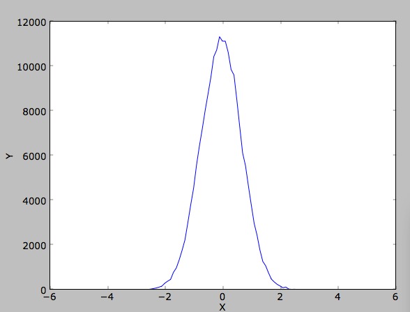
This should produce a gaussian curve with a standard deviation of 3.0. Check to make sure this is the case before going on! Now, use your histogram class to compute the density in the direction of the hydrogen molecules bond. You should expect to see something like this (if you make enough VMC steps!):

One of the most important quantities in quantum Monte Carlo is the average energy. The average energy is defined as $\langle H\Psi / \Psi \rangle \equiv \langle E_L \rangle.$ Therefore, we need to compute the local energy $E_L$. Recall that $\frac{H\Psi}{\Psi} = \frac{(-\nabla^2/2 + V)\Psi}{\Psi}$. The $(V\Psi)/\Psi$ term is relatively easy to evaluate as it just reduces to $V(r)=-\sum_{Ie} \frac{1}{r_{Ie}} + \sum_{ee} \frac{1}{r_{ee}}+\sum_{II}\frac{1}{r_{II}}$ (for a system of electrons (e) and Ions (I)). While in a real code, we would want have analytic derivatives for the $\nabla^2 \Psi / \Psi$ term, in this tutorial we will focus on just computing it with finite differences (in any case, it's important to have it computed with finite differences to check your analytic derivatives). Let's add a function, then, that takes a wavefunction, and a coordinate array and then returns the kinetic energy component of the local energy. In other words, implement the functions

def LaplacianPsiOverPsi(wavefunction,coords,ions):
  #this should return the kinetic piece 
  # of the local energy
def LocalEnergy(wavefunction,coords,ions):
  # this should return the local energy. 

Remember that $\frac{\partial^2 F}{\partial x^2} \approx \frac{F(x+\delta)+F(x-\delta)-2F(x)}{\delta^2}$

To verify that your code is correct, set your ions so that the bond length is 1.4 and set the coordinates via

R=numpy.zeros((2,3),float)
R[0]=[1.0,0.3,0.2]
R[1]=[2.0,-0.2,0.1]

You should end up with the total local energy being -1.819

Now add the calculation of the local energy to your VMC function. Have the VMC function return a list of energies. Once you have these energies, use the statitistical package to compute the energy and error as well as plotting the energies.

You should end up seeing a plot like:


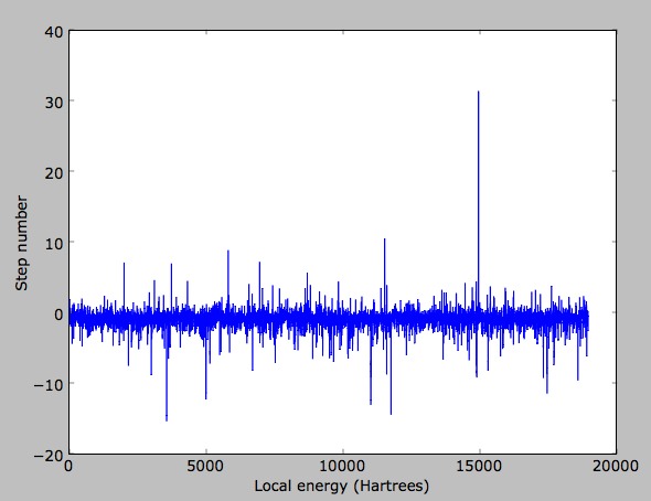
You should notice a couple things about this plot

1. It is quite spiky.
2. If you compute the statistics of your energy list, your answer is around -0.86.
3. Your variance is large.

Let's take stock of where we are. We have the functions

 psi(coords,ions)
 LaplacianPsiOverPsi(wavefunction,coords,ions)
 LocalEnergy(wavefunction,coords,ions)

Currently $\alpha$ is hard coded into these wavefunctions, but in a minute we will want to vary it! This means that we either have to make $\alpha$ a global variable (ugly!), add another parameter alpha to all these functions, or bundle the wave functions into a class. The latter of these is the most elegant solution. Imagine we define the following class:

class WaveFunctionClass:
  def psi(self,coords):
    #stuff here
  def LaplacianPsiOverPsi(self,coords): 
    #stuff here
  def LocalEnergy(self , coords):
    #stuff here
  def SetIons(self,ions):
    # stuff here
  def SetAlpha(self,alpha):
    #stuff here

Notice, that we don't have to pass around as many things (like alpha and the ions) and we still get away with not have ugly global variables. Of course, this means that you're going to have to play around with some of the function calls and such that you have in your code so far. Go ahead and make the changes in your code necessary to be using this class. (Looking through the section "Computing the density" is probably helpful now)

You should be able to test your modifications to your class with the following code (which should work if you have only the HistogramClass and the WaveFunctionClass in your file!):

import stats
wf=WaveFunctionClass()
wf.SetIons(numpy.array([[0.7,0.0,0.0],[-0.7,0.0,0.0]]))
wf.SetAlpha(0.5)
print "Psi should be 0.496585 when given coords as numpy.array([[1.0,0.5,0.3],[-0.2,0.1\
,-0.1]) and is ",wf.psi(numpy.array([[1.0,0.5,0.3],[-0.2,0.1,-0.1]]))
R=numpy.zeros((2,3),float)
R[0]=[1.0,0.3,0.2]
R[1]=[2.0,-0.2,0.1]
print  "The local energy should be -1.819 and is ",wf.LocalEnergy(R)
print "The acceptance ratio of this VMC run should be about 0.323 and plot the density \
as above"
eList=VMC(wf,10000)
myStats=stats.Stats(numpy.array(eList))
print "Your statistics should be approximately  (-0.885, 1.325, 0.028, 5.613)",myStats

Note: If you are running low on time, feel free to skip this section

30% isn't a bad acceptance ratio. It turns out we can do much better though! Recall that the acceptance ratio for Monte Carlo goes as $A(R \rightarrow R') = \min \left[\frac{\pi(R')}{\pi(R)}\frac{T(R' \rightarrow R)}{T(R \rightarrow R')} ,1 \right]$ where, in our calculation, we have that $\pi(R) = |\Psi(R)|^2$.

Now let us define that quantum force $F(R) \equiv \frac{\nabla \Psi(R)}{\Psi(R)}$. Then choose a new point $R'$ with probability $P(R') = \exp[-(R-R'-\tau F(R))^2/(4\lambda\tau)$. Notice that this will produce a non-trivial value for both $T(R \rightarrow R')$ and $T(R' \rightarrow R)$. If you implement this new Monte Carlo move, you will find that the acceptance ratio (for small $\tau$) will be approximately 1. Try modifying your VMC method to use this quantity:

Hints about implementing this:

• The biggest difficulty is implementing $\nabla \psi / \psi$. Remember that this quantity is a vector.

You may have noticed that your code is slow!! This is because you've written it in python. Even so, you can do some things to speed up your code.

• Switch the numerical derivatives to analytic derivatives. Numerical derivatives are really slow!
• Do wave function updates for single particle moves
• Pythonize it: We have been writing in python but not in a very pythonic way. 'for loops' are really slow in python. On the other hand, list comprehensions and matrix operations are much faster. Find the slow parts of your code and speed them up!
• Use cython! Cython is essentially a version of python that allows you to add types and speed up python. (Some python features don't work, though).
• Well, python is slow. Maybe you should try C++ (or fortran or fortress or ocaml).

Challenge: Think you have a particularly fast code? Time it and add it to our leader board of fast python (or other language) codes. Even better: contribute your fast code (in whatever language) as an example of a well written fast VMC code.

---

Now, we have learned how to compute integrals using Variational Monte Carlo. Often, though, we don't know what our wave function actually is (in this case, we don't know what the correct value of $\alpha$ is). In the next section, we will use the variational principle to select the best value of the paramaters. Once we've started learning how to optimize, then we can afford to make our wave function more complicated!

Continue onto the next section...